Usage
Requirements
Nothing fancy, just python 3.5.2+ and pip.
Installation
Install directly from github
git clone https://github.com/bondyra/pyBreakDown
cd ./pyBreakDown
python3 setup.py install  # (or use pip install . instead)
Basic usage
Load dataset
from sklearn import datasets
x = datasets.load_boston()
data = x.data
feature_names = x.feature_names
y = x.target
Train model
train_data = data[1:300,:]
train_labels=y[1:300]
model = model.fit(train_data,y=train_labels)
Explain predictions on test data
#necessary imports
from pyBreakDown.explainer import Explainer
from pyBreakDown.explanation import Explanation
#make explainer object
exp = Explainer(clf=model, data=train_data, colnames=feature_names)
#make explanation object that contains all information
explanation = exp.explain(observation=data[302,:],direction="up")
Text form of explanations
#get information in text form
explanation.text()
Feature                  Contribution        Cumulative
Intercept = 1            29.1                29.1
RM = 6.495               -1.98               27.12
TAX = 329.0              -0.2                26.92
B = 383.61               -0.12               26.79
CHAS = 0.0               -0.07               26.72
NOX = 0.433              -0.02               26.7
RAD = 7.0                0.0                 26.7
INDUS = 6.09             0.01                26.71
DIS = 5.4917             -0.04               26.66
ZN = 34.0                0.01                26.67
PTRATIO = 16.1           0.04                26.71
AGE = 18.4               0.06                26.77
CRIM = 0.09266           1.33                28.11
LSTAT = 8.67             4.6                 32.71
Final prediction                             32.71
Baseline = 0
#customized text form
explanation.text(fwidth=40, contwidth=40, cumulwidth = 40, digits=4)
Feature                                 Contribution                            Cumulative
Intercept = 1                           29.1                                    29.1
RM = 6.495                              -1.9826                                 27.1174
TAX = 329.0                             -0.2                                    26.9174
B = 383.61                              -0.1241                                 26.7933
CHAS = 0.0                              -0.0686                                 26.7247
NOX = 0.433                             -0.0241                                 26.7007
RAD = 7.0                               0.0                                     26.7007
INDUS = 6.09                            0.0074                                  26.708
DIS = 5.4917                            -0.0438                                 26.6642
ZN = 34.0                               0.0077                                  26.6719
PTRATIO = 16.1                          0.0385                                  26.7104
AGE = 18.4                              0.0619                                  26.7722
CRIM = 0.09266                          1.3344                                  28.1067
LSTAT = 8.67                            4.6037                                  32.7104
Final prediction                                                                32.7104
Baseline = 0
Visual form of explanations
explanation.visualize()
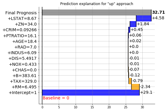
png
#customize height, width and dpi of plot
explanation.visualize(figsize=(8,5),dpi=100)
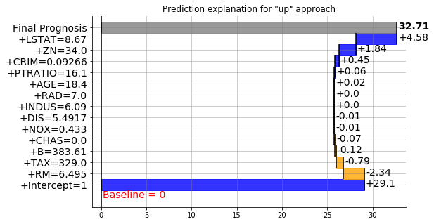
png
#for different baselines than zero
explanation = exp.explain(observation=data[302,:],direction="up",useIntercept=True)  # baseline==intercept
explanation.visualize(figsize=(8,5),dpi=100)
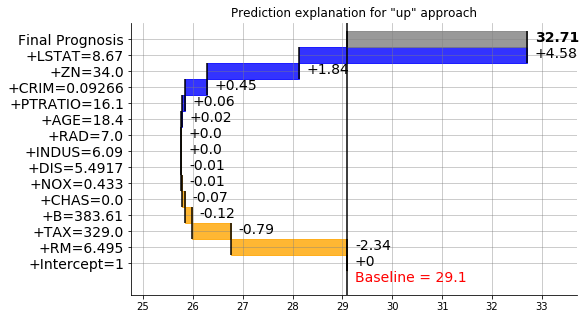
png